An introduction to closed and open chain manipulators

Course index Blackboard

n-link planar serial chain robots

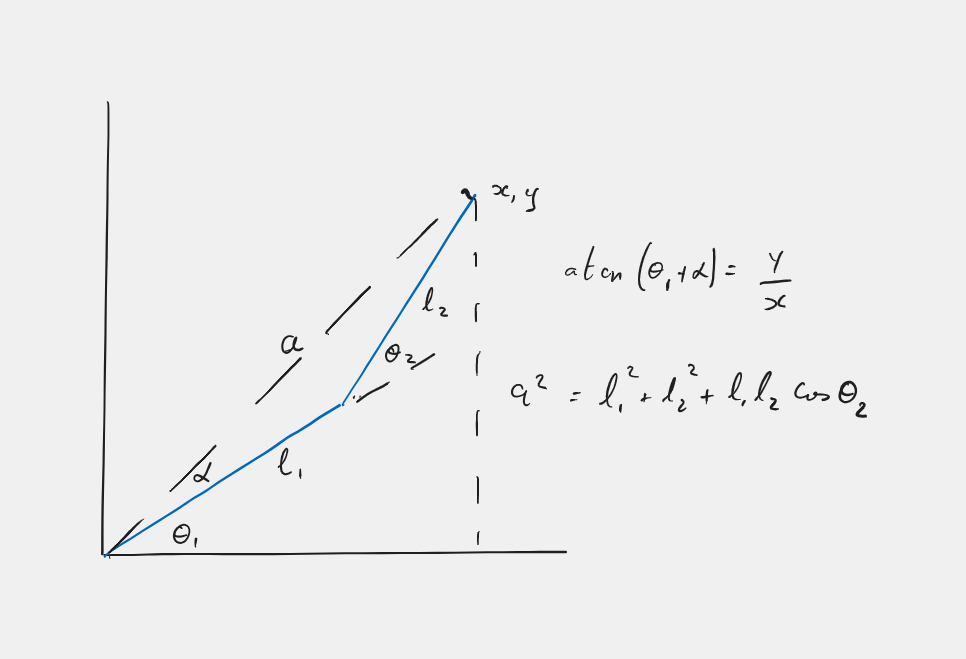
From the figure above we can write the coordinates of each of the joints $j$ as

\begin{equation} \vec{x}^T=\vec{l} F(\vec\theta) \label{fig:fk1} \end{equation}

where

\[ \vec{l}= \begin{bmatrix} l_{1} & l_{2} & l_{3} \end{bmatrix} \]

is a vector of linklengths

In addition we need to define

\[ F(\vec\theta)= \begin{bmatrix} c_{1} & s_1 \\ c_{12} & s_{12}\\ c_{123} &s_{123} \end{bmatrix} \]

where \(c_{1} =\cos\theta_{1}\), \(s_1 = \sin\theta_{1}\), $c_{12} = \cos\left(\theta _{1}+\theta _{2}\right)$, $s_{12} = \sin\left(\theta _{1}+\theta _{2}\right)$ $c_{123} = \cos\left(\theta _{1}+\theta _{2}+\theta _{3}\right)$, etc

Fortunately Matlab has a convenient function for computing successive sums called cumsum

You can cross check with the above figure by using following Matlab code Note this gives you the symbolic solution!

>> syms theta1 theta2 theta3 l1 l2 l3 real
>> theta=[theta1; theta2; theta3]
>> l=[l1 l2 l3]
>> F=[cos(cumsum(theta)) sin(cumsum(theta))]
>> x=l*F


It is also possible to use an anonymous function in Matlab to compute the position of the end of the last link

The forward kinematics of any number of links can be done with the anonymous function

>> fk=@(len,theta) len*[cosd(cumsum(theta)) sind(cumsum(theta))];


Where $len$ is a vector of link lengths and $theta$ is a vector of angles.

the length of the vectors len and theta must be the same (and theta must be in degrees) but this function will work for any number of links in an open (serial) chain.

Generalised n-link

The generalisation to n-links is ....

\begin{equation} \vec{x}=L F(\vec\theta) \label{fig:fk2} \end{equation}

where L is a matrix of linklengths such that

\[ L= \begin{bmatrix} 0 & 0 & 0\\ l_{1} & 0 & 0\\ l_{1} & l_{2} & 0\\ l_{1} & l_{2} & l_{3} \end{bmatrix} \]

and

\[ F(\vec\theta)= \begin{bmatrix} \cos\theta_{1} & \sin\theta_{1}\\ \cos\left(\theta _{1}+\theta _{2}\right) & \sin\left(\theta _{1}+\theta _{2}\right)\\ \cos\left(\theta _{1}+\theta _{2}+\theta _{3}\right) & \sin\left(\theta _{1}+\theta _{2}+\theta _{3}\right) \end{bmatrix} \]

This technique can be extended readily to give the locations in the base coordinate frame of each joint and hence to draw the pose of the linkage.

plot with

>> x=L*F
>> plot(x(:,1),x(:,1))


Inverse kinematics

Inverse kinematics is the challenge of calculating the joint angles needed to get to a specific position.

From equation 1 you can see that the end point vector can be written as a function of the joint angle vector.

• If you want the robot to be in a particular position how might you calculate the joint angles?
• How many solutions are there for a 2-link chain?
• How many solutions are there for a 3-link chain?

Calculating the inverse kinematics the difficult way

Calculating the inverse kinematics the lazy way

• This is a numerical method
• May fail because
  • of numerical instability (stiff equations)
  • there is no solution
  • run out of time
  • the error surface is flat

1. Fix the constants, in this case lengths, and calculate forward kinematics

>> len=[1.6 1.8];
>> fk=@(theta) len*[cosd(cumsum(theta)) sind(cumsum(theta))];


2. Specify the target position

>> xtarget=[0 2.1];


3. Work out an errorfunction

• Should be always positive,
• Should get smaller as it gets close to the target position

>> errfn=@(theta) (xtarget-fk(theta))*(xtarget-fk(theta))';


The way this works is we create a vector [dist_in_x, dist_in_y] and use a matrix operation that means

\[ \begin{bmatrix}d_x & d_y \end{bmatrix} \begin{bmatrix}d_x \\ d_y \end{bmatrix} =d_x^2+d_y^2 \]

4. Check that the error function is sensible

>> errfn([70;0])'
>> errfn([70;20])'


5. Use the Nelder-Mead simplex algorithm (or any other way) to find minimum or maximum of a function.

>> [X,fval]=fminsearch(errfn,[45;45])


6. Check

>> L=[0 0;len(1) 0;len];
>> x=L*[cosd(cumsum(X)) sind(cumsum(X))]
>> plot(x(:,1),x(:,2));axis('equal');grid on