Biological Cybernetics: Non-Linear systems
\\
There may be additional information on the websites
Assessment is via examination and one assignment (to be posted on blackboard)
The assignment will be set in December with the submission on 13th January 2023
Autumn labs at 11am in PV184 on Tue 15-11-2022 and Tue 29-11-2022
The following books are some of the references used in the course
Start with the identity
\begin{equation} a=\frac{d^2x}{dt^2}=\frac{dv}{dt}=\frac{dv}{dt}\frac{dx}{dx}=v\frac{dv}{dx} \label{eq:suvat} \end{equation}Rewrite to as
\[ a dx= v dv \]Assume that $a$ is constant and that we can integrate from some initial condition $x_0$,$v_0$ to some final condition $x_{(t)},v_{(t)}$
\[ a \int^{x(t)}_{x_0} dx=\int^{v(t)}_{v_0} v dv \]After integration and substitution we get
\[ a(x-x_0)=\left(\frac{v^2}{2}-\frac{v_0^2}{2}\right) \]Sketch trajectories on phase-plane as parabolas.
Cybernetics: The scientific study of control and communication in the animal and the machine. Norbert Wiener 1948
... which I call Cybernétique, from the word $\kappa\nu\beta\epsilon\rho\nu\varepsilon\tau\iota\chi\eta$ which at first (taken in a limited sense) is the art of governing a vessel but (even among the Greeks) extends to the art of governing in general.[ampere38:essai] André-Marie AmpèreThe ancient Greek word kybernetikos ("good at steering"), refers to the art of the helmsman.
Latin word guberno/gubernãre that is the root of words for government comes from the same Greek word that gives rise to cybernetics.
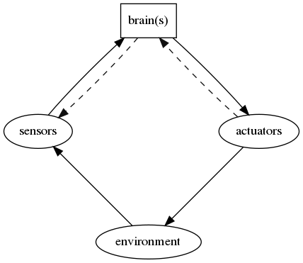
The possession of a brain allows humans, animals and (to some extent) robots to have a meaningful interaction in a complex environment. Intelligence may be observed from the way we react in this environment but (as shown in figure below), sense our environment and use this information to update internal models we have of the world. We react to this information via our understanding of the behaviour of our internal models and operate through muscles to enable us to alter our environment to our benefit.
Other relevant concepts
Highly recommended Ted Talk (https://www.ted.com/talks/daniel_wolpert_the_real_reason_for_brains) Daniel Wolpert. The real reason for brains. March 2014
A system is an object that we would like to study, control and affect the behaviour.
A model is the knowledge of the properties of a system. It is necessary to have a model of the system in order to solve problems such as control, signal processing, system design. Sometimes the aim of modelling is to aid in design. Sometimes a simple model is useful for explaining certain phenomena and reality.
A model may be given in any one of the following forms:
Most systems we are interested in are expressed with differential equations if they are continuous, and difference equations if they are sampled.
A value $y(t)$ exists at all points values of $t$ (or more usually all points in $t\ge 0$)
This should also be true of all derivatives of $y$
A value $y(n)$ exists only at specific times, that is at all positive integer values of $n$. It may be convenient to occasionally include 0 or negative integers in $n$.
Tend to be defined in terms of a delay operator $q^{-1}$ such that for a sequence $u(i)$ the operator delays each value by one timestep, i.e. $q^{-1}u(i)=u(i-1)$. The $q$ operator is interchangeable with the $z$ transform.
How might differentiation and integration be done in a sampled time data
If $y=f(u(t))$ is a system (or function) with an input $u(t)$ that can change with time $t$ then the system can be considered as linear if
\[ y'=f(a u(t))=a y \]for some constant scalar value $a$.
This applies also to the vector form i.e. if $\vec{y}=f(\vec{u})$ then the system can be considered as linear if
\[ a\vec{y}=f(a\vec{u}) \]The concept of state space has two benefits, first it allows a system to be described as a vector of states such as position, velocity, voltage, current etc. Second it allows the equations (both linear and non linear) to be written as a single level of differentiation.
The general form for a state space with states $\vec{x}(t)$, inputs $\vec{u}(t)$ and outputs $y(t)$ is
\begin{align} \dot{\vec{x}}&=f(\vec{x},\vec{u},t)\\ \vec{y}&=g(\vec{x},\vec{u},t) \label{eq:nonlinCD} \end{align}with input $\vec{u}$, output $\vec{y}$ and states $\vec{x}$. All variables are assumed to be a function of $t$.
Linear state space equations are often written with the ABCD notation
\begin{align} \dot{\vec{x}}&= A \vec{x} +B\vec{u}\\ \vec{y}&= C\vec{x}+D\vec{u} \label{eq:linCD} \end{align}With constant matrices $A,B,C,D$
Often, in both linear and non-linear versions, the equations above are simplified to $\vec{y}= C\vec{x}$ with C being an identity matrix.Matlab ("matrix laboratory") is a programming language for numerical computing, that provides an extensive set of tools and libraries, a relatively readible structure, and good graphics in 2 and 3 dimensions. Matlab also provides a graphical language (simulink) for system analysis and a symbolic maths package based on Mupad. The numerical parts of this course will be based on Matlab and it is recommended that you use this for the second assignment.
Mathworks courses on matlab are
Matlab Onramp (2 hours) Mathworks.
Matlab Fundamentals, Mathworks
Other courses are
Learning Matlab (1h13m) Steven Moser, Linkedin learning
MATLAB 2018 Essential Training (3h15m) Curt Frye, Linkedin learning
The university has a Matlab licence for all students. But many of the tools are available through other packages (albeit not as good). Some alernatives are
Method 1: AppsAnywhere: https://www.reading.ac.uk/internal/its/AppsAnywhere.aspx
Method 2: Create an account at mathworks.com using your student email address. (https://uk.mathworks.com/mwaccount/) (https://www.reading.ac.uk/internal/its/services/its-SerCat/MatlabStudents.aspx) Download MATLAB (Individual)
A simple first order system tends to be in the form $\displaystyle \frac{dy}{dt}+k y=0 $ or
\[ \dot{y}+k y=0 \]where $k$ is a constant
The solutions are of the form
\begin{equation} y=e^{at} Y_0 \label{eq:simplefirst} \end{equation}where $y_0$ is an initial condition. It is possible to see that this is a good guess by differentiating eq t.b.d. (eq:simplefirst) and comparing coefficients.
Substitute the solution into the first order equation we get
\[ \left(ae^{at}+k e^{at}\right)Y_0=0 \]so $a=-k$ is the solution is
\[ y=e^{-kt}Y_0 \]when there is a non zero initial condition for $Y_0$. Set $t=0$ in equation t.b.d. (eq:simplefirst) to confirm the initial condition is $Y_0$
It is also possible to get a solution with the Laplace transform in which case the first order equation has the Laplace transform
\[ (sy-Y_0)+k y=0 \]again with $Y_0$ the initial condition, i.e. the value of $y$ at $t=0$
A first order system can have an input driving the response. These are of the form
\[ \frac{dy}{dt}+k y=u \]where $u$ is an input variable. The solution is slightly more complicated and for an arbitrary input the solution would be solved by numerical integration. Some specific inputs can be calculated so for a 'step change' the solution is of the form
\[ y=U_0\left(1-e^{-kt}\right) \]where $U_0$ is the size of the step.
Second order systems are widely used for modelling e.g.
A general form of an equation that describes a second order system is
\begin{equation} \frac{d^2y}{ dt^2}+\beta\frac{dy}{dt}+\omega^2 y=0 \label{eq:soss} \end{equation}where $\beta$ (beta) and $\omega$ (omega) are constant values convenient to write $\beta=2\zeta\omega$ ($\zeta$ is zeta). A second order system can then be described as having a natural frequency $\omega$ or $\omega_n$ (in radians per second) and a damping ratio $\zeta$. If zeta is 0 then the second order system will oscilate at $\omega_n$ and if zeta is equal to 1 the second order system will come to rest in the shortest time.
Equation t.b.d. (rq:soss) can also be written in a 'state space' form, ie as a matrix equation. This can be expressed by letting $x_1 \equiv y$ and $x_2 \equiv dy/dy$ so
\[ \begin{bmatrix}\dot{x_1}\\\dot{x_2}\\\end{bmatrix} = \begin{bmatrix}0 & 1\\-\omega^2&-\beta\end{bmatrix} \begin{bmatrix}{x_1}\\{x_2}\\\end{bmatrix} \]i.e. $\vec{\dot{x}}=A\vec{x}$ where $\displaystyle A=\begin{bmatrix}0 & 1\\-\omega^2&-\beta\end{bmatrix} $
We can check this by substituting back
\[ \begin{bmatrix}\frac{dy}{dt}\\\frac{d^2y}{dt^2}\\\end{bmatrix} = \begin{bmatrix}\dot{x_1}\\\dot{x_2}\\\end{bmatrix} = \begin{bmatrix}0 & 1\\-\omega^2&-\beta\end{bmatrix} \begin{bmatrix}{y}\\\frac{dy}{dt}\\\end{bmatrix} \]The solution to this is very similar to that for the first order solution. It is
\[ \vec{y}=e^{-At}\vec{Y}_0 \]Although we need to define a matrix version of an exponent which we will do in the lab.
A mechanical example is a mass connected to a spring and damper

By equating forces on the mass $m$ it is possible to derive the free running system as
\[ m\ddot{x}+c\dot{x}+k x=0 \]or the force driven system as
\begin{equation} m\ddot{x}+c\dot{x}+k x=f \label{eq:massspring} \end{equation}Equation \eqref{eq:massspring} can also be written as
\[ \ddot{x}+\frac{c}{m}\dot{x}+\frac{k}m x=\frac{f}{m} \]so it is then possible to see that $\omega^2=\frac{k}{m}$ and $\beta=2\zeta\omega=\frac{c}{m}$
See (http:w8interactive.html)Recall that for a square matrix $A$ the Eigenvectors $v$ are special vectors that when real have the same direction when transformed by A.
So if
\[ v'=A v \]then $v$ is an Eigenvector if $v'=\lambda v$. i.e.
\begin{equation} Av=\lambda v \label{eq:eigval} \end{equation}The same is true if the Eigenvectors are complex, but it is may be harder to conceptulise a complex scaling value $\lambda$ and complex direction of $v$. One additional cavet is that if the Eigenvalue is real and negative then $v'$ will point in exactly the oposite direction to $v$, that is to say it now as negative magnitude.
From the equation \eqref{eq:eigval} above we can compute a solution by noting that
\[ (A-\lambda I)v=0 \]and by realsing that for any non zero vector $v$ the matrix $A-\lambda I$ must be singular and in which case the determinant must be zero hence
\[ \begin{vmatrix}A-\lambda I\end{vmatrix} = 0 \]The stability of the system is dictated by the Eigenvalues of the $A$ matrix, more specifically whether the real parts of the Eigenvalues are greater than zero. For a second order system (where we use the substitution $\beta=2\zeta\omega$) the the Eigenvalues are
\[ \lambda=-\omega(\zeta \pm\sqrt{\zeta^2 - 1}) \]Now omega ($\omega$) only effects the magnitude of the Eigenvalues, so we can map out the behaviour of the system based on the value of zeta ($\zeta$).
| zeta | lambda ($\lambda$) | behaviour |
| $\zeta<-1$ | real positive numbers | exponentially increasing (unstable) |
| $-1<\zeta< 0$ | complex with positive real part | increasing oscillations (unstable) |
| $\zeta=0$ | imaginary (real part is zero) | stable oscillations |
| $0<\zeta< 1$ | complex with negative real part | decreasing oscillations (stable) |
| $\zeta>1$ | real negative numbers | exponentially decreasing (stable) |
A simple model of biped walking is based on an 'inverted pendulum'. The assumption is that during the period you have one foot on the ground your knee is 'locked' and your dynamics are similar to a pendulum that can swing in two dimensions [kajita01].

By analysing the forces on a pendulum (left figure), or equivalently the accelerations (right figure) we can derive the pendulum equations. Either way the non-linear pendulum equation is then
\[ \ddot\theta=-\frac{g}{l}\sin\theta \]This can also be written in state space form as
\begin{align} \dot\theta&=\omega\\ \dot\omega&=-\frac{g}{l}\sin\theta \end{align}Where we introduce the additional state variable omega \[\omega=\frac{d\theta}{dt}\]
We can find a numerical solution to the above state-space equation using 'ode' integrators such 'Euler' or 'Runge-Kutta'.
There is also an analytic approach that can be used to draw and understand the phase plane.
This uses a refactoring of a second differential. If we write $\dot{x}=\frac{dx}{dt}=v$
\[ \ddot{x}=\frac{dv}{dt}=\frac{dv}{dx}\frac{dx}{dt}=\frac{dv}{dx}v \]If we replace $x$ and $v$ in the above equation for $\theta$ and $\omega$ we can substitute that into the non-linear pendulum equation so
\[ \omega\frac{d\omega}{d\theta}=-\frac{g}{l}\sin(\theta) \]Rewrite to get
\[ \omega d\omega=-\frac{g}{l}\sin(\theta){d\theta} \]and integrate with the limits of each integral corresponding.
\[ \int_{\omega(0)}^{\omega(t)}\omega d\omega=-\int_{\theta(0)}^{\theta(t)}\frac{g}{l}\sin(\theta){d\theta} \]Once the integration is done and the limits evaluated the equation becomes
\[ \frac12\left(\omega^2(t)-\omega^2(0)\right)= \frac{g}{l}\left(\cos\theta(t)-\cos\theta(0)\right) \]
So it is then possible to rearrange to compute $\omega(t)$ from the initial conditions $\omega(0)$ and $\theta(0)$ and the current angle $\theta(t)$ That is
\[ \omega(t)= \pm\sqrt{ \frac{g}{l}\left(\cos(\theta(t))-\cos(\theta(0))\right) +\omega^2(0) } \]Since this is no longer time dependent we can write it as
\begin{equation} \omega= \pm\sqrt{ \frac{g}{l}\left(\cos\theta-\cos\theta_0\right) +\omega^2_0 } \end{equation}Challenge is to plot $\omega$ vs $\theta$ for a variety of angles
where $l$ and $m$ the pendulum length and mass, in this case the constant $B$ is known as damping (inherent energy loss) of the system, and $g$ is gravitational acceleration.


Closed form solution if $B=0$
Assuming $\dot{x}=v$ Can use the relationship
\[ \frac{d^2 x}{dt^2}= \frac{dv}{dt}= \frac{dv}{dx}\frac{dx}{dt}= \frac{dv}{dx}{v} \]Now do the equivalent calculation for $\dot\theta=\omega$ and solve equation t.b.d. (eq:pend1)
We will cover only Initial value problems, i.e we are interested in looking at the behaviour of a 'thing' as it evolves over time.
Tend to be set out for problems of the form
\[ \dot{\vec{x}}=f(t,\vec{x}) \]Sometimes expressed with a mass matrix
\[ M(t,\vec{x})\dot{\vec{x}}=f(t,\vec{x}) \]Note: Numerical solvers will often adapt the step-size to the problem and can use additional information, such as problem constraints or higher order differentials. Solver also needs to know the initial value. System inputs can be included in the process.
Note2: Stiff solvers may be needed for problems where there is a strong coupling between state variables. (e.g. the Robertson's chemical reaction (use your favourite search engine to find out more))
Suppose we know the continuous time state-space equations for a system.
\[ \dot{x}=f(\vec{x})+g(\vec{u}) \]For the moment we will consider $f$ and $g$ non-linear functions, although we can always revert them to being matrices $A$ and $B$ if they system is linear.
Approximate this as
\[ \dot{\vec{x}}\approx \frac{\vec{x}(t+\Delta)-\vec{x}(t)}{(t+\Delta)-t} =f(\vec{x}(t))+g(u(t)) \]the $t$ in the denominator cancel so we can rearrange the equation to be
\[ \vec{x}(t+\Delta)=\vec{x}(t) +\Delta f(\vec{x}(t))+\Delta g(u(t)) \]If we set $\Delta$ to be fixed this is then a sampled data system so we can effectively integrate the states. If we ignore the input for the moment, and accept that $\vec{x}$ is a function of time, we get
\[ x_{n+1}=x_{n}+\Delta f(x_{n}) \]And if the system is linear then $f(\vec{x})$ becomes $A\vec{x}$ which is simply a fixed matrix so the equation becomes
\[ x_{n+1}=x_{n}+\Delta A x_{n} \]note: Forward Euler is known to be poor, but is often used in real-time software. Delta needs to be small to be effective, but this is then expensive in computer time.
challenge: use the $q$ operator to rewrite this equation, and then see if you can sketch it out as a transfer function and as a code fragment.
If we look at the approximation for the Forward Euler case (and assuming it is linear with no input), we may be able to write it as
\[ \frac{\vec{x}(t)-\vec{x}(t-\Delta)}{t-(t-\Delta)} =f \vec{x}(t) \]or
\[ \vec{x}(t)=\vec{x}(t-\Delta)+\Delta f \vec{x}(t) \]Again if $\Delta$ is constant we can consider this as a sampled data system.
\[ x_{n}=x_{n-1}+\Delta f(t_{n},x_{n}) \]Effectively now are looking backwards in time for the state, but we have already computed the state! This may be possible for some systems but in most cases we will look for more sophisticated numerical integrators, such as Runge Kutta
(Here we change from using $\vec{x}$ as a vector of states to $y$ that can also be a vector of states - that way we don't need to change the wikimedia figure!)
$\dot {y}=f(t,y)$ with initial values $y(0)=y_{0}$.

For a positive step size h compute in order the following values of the function to be integrated (i.e. the function gradients)
You now have 4 gradients as shown inThe function estimate used as the result is then
\begin{align} y_{1}&=y_{0}+h{\frac{1}{6}}\left(k_{1}+2k_{2}+2k_{3}+k_{4}\right)\\ t_{1}&=t_{0}+h \label{eq:sample} \end{align}See\eqref{eq:sample}
Repeat for the new values of $t_1$ and $y_1$ so in general
\begin{align} y_{n+1}&=y_{n}+h{\frac {1}{6}}\left(k_{1}+2k_{2}+2k_{3}+k_{4}\right)\\ t_{n+1}&=t_{n}+h \end{align}Where $k_1, k_2, k_3$ and $k_4$ are defined by the figureIf we have a state space model we can choose any two states and map out the state gradients with all other states fixed.
If we assume the general form of a non-linear model with two states of the form
\[ \begin{bmatrix}\dot{x}_1\\\dot{x}_2\end{bmatrix} =f\left(\begin{bmatrix}x_1\\x_2\end{bmatrix}\right) \]If our phase space has axes for $x_1$ (horizontal) and $x_2$ (vertical) we can, for every point on the $x_1,x_2$ plane, compute the gradient of the trajectory.
This gradient is $\frac{d x_2}{d x_1}$ and we can expand it so
\[ \frac{d x_2}{d x_1}=\frac{d x_2}{d x_1}\frac{d t}{d t} = \frac{d x_2}{d t}\frac{d t}{d x_1} = \frac{d x_2}{d t}/\frac{d x_1}{d t} = \frac{\dot{x}_2}{\dot{x}_1} \]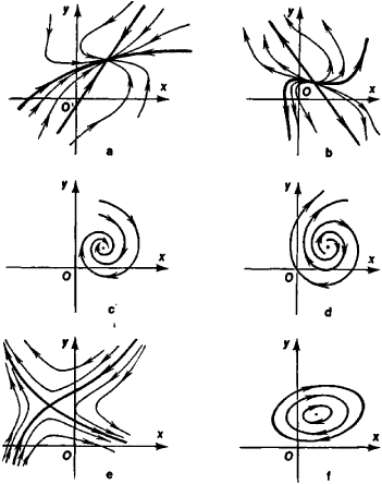
There are many non-linear system models, using a variety of techniques to model dynamics. The following is a sample of a few that are based on non-linear differential equations.
See earlier
This is an efficient spiking model of a Neuron proposed by Eugene Izhikevich in his paper "Simple Model of Spiking Neurons" IEEE Transactions on Neural Networks (2003) 14:1569- 1572
Izhikevich uses a simple Euler integrator.
\begin{align} \dot{v}&=e v^2+f v +g -u +I\\ \dot{u}&=a(bv-u) \end{align}$v$ represents the membrane potential, $u$ represents the neuron recovery (related to the flux of potassium post firing) $I$ is treated as an input current and either excites or inhibits the neuron.
if $v \ge 30$, then $v$ resets so $v=c$ and $u$ resets to $u+d$.
$a, b, c, d, e, f$ and $g$ are constants that depend on the type of neuron. Typically $e=0.04$, $f=5$, $g=140$. The parameters $a$, $b$, $c$, $d$ are chosen to represent differing neurons as per figure t.b.d. (fig:izhikevich2)

The van der Pol equation (with zero input) expressed as a second order single equation is
\[ \frac{d^2y}{ dt^2}-\mu(1-y^2)\frac{dy}{dt}+y=0 \]where $\mu$ is a constant value that controls behaviour.
Some observations are:
We can express the van der Pol equations in a state space form
\[ \begin{bmatrix}\dot{x_1}\\\dot{x_2}\\\end{bmatrix} = \begin{bmatrix}0 & 1\\-1 & \mu (1-x_1^2)\end{bmatrix} \begin{bmatrix}{x_1}\\{x_2}\\\end{bmatrix} \]Although this looks like a linear system this is not the case. Why? (are all the values in the $A$ matrix constants?)


Local gradients can be calculated at all points in the phase plane since
\[ \frac{dx_2}{dx_1}= \frac{dx_2}{dt}\frac{dt}{dx_1}= \frac{\dot{x}_2}{\dot{x}_1} \]So for the van der Pol oscillator the local gradient for any point can be computed as
\[ \frac{dx_2}{dx_1} =\frac{\dot{x}_2}{\dot{x}_1} =\frac{ - x_1 +\mu (1-x_1^2) x_2}{x_2} \]The above conditions are now
The Lorenz equations were the first evidence of chaotic system. They were originally a description of the convection in clouds, but are now seen as one of the classic examples of a system that exhibits chaotic and predictable behaviour, depending on the parameter values of the model.
\begin{align} \frac{\mathrm{d}x}{\mathrm{d}t} &= \sigma (y - x), \\ \frac{\mathrm{d}y}{\mathrm{d}t} &= x (\rho - z) - y, \\ \frac{\mathrm{d}z}{\mathrm{d}t} &= x y - \beta z. \end{align}Classically Lorenz equations used the values ${\displaystyle \sigma =10}, {\displaystyle \beta =8/3}$ and ${\displaystyle \rho =28}$. when the system is chaotic.
The Lotka–Volterra model are a very simple two species population model describing prey that expand their population exponentially, and predators that expand their population as a function of the number of available prey.
\[ \begin{aligned}{\frac {dx}{dt}}&=\alpha x-\beta xy,\\{\frac {dy}{dt}}&=\delta xy-\gamma y,\end{aligned} \]If $x$ are the pray and $y$ are the predators, then the constants in the above equation can be considered to mean the following.
These equations exhibit classic limit cycles. In the absence of predators the prey population increases. As more prey become available, the predictor population increases. Too many predators eat the prey and the prey population decreases. Since there are fewer prey to eat the predators die of starvation.
Lotka-Volterra is readily graphed in Matlab with an inbuilt function
\includegraphics[width=0.95\textwidth]{html/lvbc.pdf}
The classic epidemic model is known as the SIRs model[ditsworth19:_infec_model]. It is an example of a compartmental model where drugs, people, things etc are considered to move at specific rates between different compartments. In the case of the SIRs epidemic model these compartments are Susceptible, Infected and Removed.
In the case of an epidemic Removed can be either because the person has recovered or has died. Thus the progression of the population is from Susceptible through to infected, and finally either recovered or died, but either way, no longer effecting the epidemic.
This model is very simplistic and, for example, does not consider vaccination rates, i.e. a flow directly from S to R, reinfection rates (flow from R to S), or additional compartments such as the number of vaccines, virus mutations, peoples behaviour etc.
There are two constants that drive the model, the contact rate ($\mathtt{C}$ or $\beta$) that controls the movement from Susceptible $S$ to Infected and the healing rate $\mathtt{H}$ or $gamma$ that controls the movement from Infected to Removed.
The SIR model is then
\begin{align} \frac{dS}{dt} &= -\mathtt{C} S I\\ \frac{dI}{dt} &= \mathtt{C} S I - \mathtt{H} I\\ \frac{dR}{dt} &= \mathtt{H} I = \dot{S}-\dot{I} \end{align}Note that $S + I + R$ is the total population and usually considered a constant. In simulations it can be set so $S + I + R=1$
The R number is the reproduction number and $R=\frac{\mathtt{C}}{\mathtt{H}}$ is the expected number of cases that will be generated per infected person in the population. Thus if a person with the disease infects more than 1 other person then the epidemic will escalate, if a person with the disease infects less than one other person the disease will die away (we can either allow fractional people, or consider this as say 100 people infecting on average R*100 other people). See also (https://en.wikipedia.org/wiki/Basic_reproduction_number)The initial value of $R$ is sometimes known as $R_0$. The management of an epidemic can be considered as finding ways to to reduce the $R$ value, ideally so that it is less than 1. Thus measures for covid19 at the moment include keeping distance, washing hands wearing face-masks. Track and trace effectively reduces the contact rate C and hence R. When a vaccine becomes available this can considered a way of removing people from $S$. Alternatively it can be considered as reducing $\mathtt{C}$. As more is learned about the management of the disease there remains an additional way to reduce R by increasing $\mathtt{H}$. Thus it is possible to influence the course of the epidemic as shown in the figure below (http:sir4.m) .


Please note in the following section we will use both the underscore/overarrow ($\vec{v}$) and bold face $\boldsymbol{\phi}$ to represent vectors.
If we have some data and a proposed model for the data the challenge is to find the parameters for that model that best represent the data. For example if you have a graph that shows the height of a person in relation to their age, you could fit a variety of models
The figure below shows scatter plots for height-age data of young women in the !Kung San culture collected in late 1960s. The linear model is of the form
\begin{equation} y=mx+c \label{eq:ymxc} \end{equation}The non-linear model is of the form
\begin{equation} y=m_1x^2 + m_2 x+c \label{eq:ymx} \end{equation}

Which model best represents the data? It may be that if we are considering individual women below the age of 20 we can use a linear regression, however if we would like a model to fit a larger population we will need to use more sophisticated models of the data, depending on this model we may still be able to fit the model with the technique of least squares regression (first proposed by Gauss in 1822).
We can write a more general form for the equations \eqref{eq:ymxc} and \eqref{eq:ymx} by putting the parameters ($m_1$, $c$ etc) into a vector variable, and creating a matrix of independent parameters $X$. In the case of equation \eqref{eq:ymx} this can be written as
\[ y=\begin{bmatrix}x^2 & x& 1\end{bmatrix} \begin{bmatrix}m_1 \\ m_2\\ c\end{bmatrix} =\begin{bmatrix}x^2 & x& 1\end{bmatrix} \boldsymbol{\theta} =\phi^T \boldsymbol{\theta} \]where $\boldsymbol{\theta}$ contains the constant values (model parameters) that we would like to fit to our data.
We can now consider our model for every data point model, it may not fit precisely so we can add a variable $e$ to account for this difference.
The simplest parametric model is linear regression.
\begin{equation} y_i={\hat y}_i+e_i= \boldsymbol{\phi}^T_i\boldsymbol{\theta}+e_i \label{eq:regress1} \end{equation}The variable $\hat{y}_i$ is known as y-hat and is the models estimate of the true result $y_i$. We may or may not also have a data point for $y_i$ which often (and confusingly) is often referred to with the same symbol. $\phi_i$ is a vector of known quantities, and $\boldsymbol{\theta}$ is a vector of unknown parameters.
We can expand the above equation for each data point, this will result in a matrix calculation that we can then solve for the parameters in $\boldsymbol{\phi}$. So
\begin{align*} y_1&={\hat y}_1+e_1= {\phi}^T_1\boldsymbol{\theta}+e_1\\ y_2&={\hat y}_2+e_2= {\phi}^T_2\boldsymbol{\theta}+e_2\\ y_3&={\hat y}_3+e_3= {\phi}^T_3\boldsymbol{\theta}+e_3\\ &\vdots\\ y_n&={\hat y}_n+e_n= {\phi}^T_n\boldsymbol{\theta}+e_n \end{align*}Forming this into a matrix we can write
\[ \begin{bmatrix}y_1\\y_2\\y_3\\\vdots\\y_n\end{bmatrix} = \begin{bmatrix}\phi^T_1\\\phi^T_2\\\phi^T_3\\\vdots\\\phi^T_n\end{bmatrix} \boldsymbol{\theta} + \begin{bmatrix}e_1\\y_2\\e_3\\\vdots\\e_n\end{bmatrix} \]or as vectors and matrices this becomes
\[ {\bf y}=X\boldsymbol{\theta}+{\bf e} \]Note that ${\bf e}$ is modelling error and this is usually assumed to be a random variable with zero mean.
Given a model form and a data set, we wish to calculate the parameter $\boldsymbol{\theta}$. One way is to minimise the errors between the actual $y_i$ and the model prediction ${\hat y}_i$.
We wish to fit a model of the form $y(t)=au(t) + b + e(t)$ with the following data
| $t$ | 1 | 2 | 3 | 4 | 5 |
| $u(t)$ | 1 | 2 | 4 | 5 | 7 |
| $y(t)$ | 1 | 3 | 5 | 7 | 8 |
We need to form the following vectors and matrices $\boldsymbol{\theta}=[a, b]^T$, $\boldsymbol{\phi}(t)=[u(t), 1]^T$. $X=\begin{bmatrix}\phi^T_1\\\phi^T_2\\\phi^T_3\\\vdots\\\phi^T_n\end{bmatrix}$
\[ \hat {\bf y}=\left( \begin{array}{c} {\hat y}_1 \\ {\hat y}_2 \\ {\hat y}_3\\ {\hat y}_4 \\ {\hat y}_5 \\ \end{array} \right)=\left( \begin{array}{cc} 1 & 1 \\ 2 & 1 \\ 4 & 1 \\ 5 & 1 \\ 7 & 1 \\ \end{array} \right)\boldsymbol{\theta}=X \boldsymbol{\theta} \]What is the correct form of the vector ${\bf y}$, where $\hat{\bf y}+{\bf e}={\bf y}$
We wish to fit a model of the form $y_i=b_2u^2_i+b_1u_i+b_0+e_i$
$\boldsymbol{\theta}=[b_2, b_1,b_0]^T$, $\boldsymbol{\phi}_i=[u^2_i, u_i, 1]^T$.
\begin{align} \hat {\bf y}&=\left( \begin{array}{c} {\hat y}_1 \\ {\hat y}_2 \\ \vdots\\ {\hat y}_{N-1} \\ {\hat y}_{N} \\ \end{array} \right)\nonumber\\&=\left( \begin{array}{ccc} u^2_1 & u_1 &1\\ u^2_2 & u_2 &1\\ \vdots&\vdots &\vdots\\ u^2_{N-1} & u_{N-1} &1\\ u^2_N & u_N &1\\ \end{array} \right)\boldsymbol{\theta} \nonumber \\ &=X\boldsymbol{\theta} \nonumber \end{align}For $i=1,...,N$,
\[ e_i=y_i-{\hat y}_i \]In vector form
\[ {\bf e}=\left(\begin{array}{c} e_1 \\ e_2 \\ \vdots\\ e_{N-1} \\ e_N\\ \end{array} \right)={\bf y} - \hat{\bf y} \]The sum of squared errors is known as SSE and is
\[ \textrm{SSE}=\sum_{i=1}^{N}e^2_i= {\bf e}^T{\bf e} \]The model parameter vector $\boldsymbol{\theta}$ is derived so that the distance between these two vectors is the smallest possible, i.e. SSE is minimised.
\begin{align*} {\bf e}^T{\bf e}=&({\bf y}-{\hat {\bf y}})^T({\bf y}-{\hat {\bf y}})\\ = &({\bf y}^T-{\hat {\bf y}}^T)({\bf y}-{\hat {\bf y}}) \end{align*}We can make the substitutions $\hat {\bf y}=X\boldsymbol{\theta}$ and $(X\boldsymbol{\theta})^T={\boldsymbol{\theta}}^TX^T$ into the above equation then expand so
\begin{align*} {\bf e}^T{\bf e}=&({\bf y}^T-\boldsymbol{\theta}^TX^T )({\bf y}-X\boldsymbol{\theta} ) \\ =&{\bf y}^T{\bf y}-2\boldsymbol{\theta}^TX^T {\bf y} +\boldsymbol{\theta}^TX^TX\boldsymbol{\theta} \end{align*}Note that the sum of squares error is a scalar value that will always be positive or zero. We would like to find the smallest sum of squares error, that is
\[ \textrm{SSE}= {\bf e}^T{\bf e}={\bf y}^T{\bf y}-2\boldsymbol{\theta}^TX^T {\bf y} +\boldsymbol{\theta}^TX^TX\boldsymbol{\theta} \]and the $\textrm{SSE}$ has the minimum when
\[ \frac{\partial (\textrm{SSE}) }{\partial \boldsymbol{\theta}}= {\bf 0} \]Differentiating the equation is relatively straight forward, even though these are matrices.
\begin{align*} \frac{\partial (SSE) }{\partial \boldsymbol{\theta}} & = - 2[\frac{\partial ( {\bf y}^TX\boldsymbol{\theta} )}{\partial \boldsymbol{\theta}} ]^T+\frac{ \partial ( \boldsymbol{\theta}^TX^TX\boldsymbol{\theta} ) }{\partial \boldsymbol{\theta}} \\ {\bf 0} &= -2 X^T{\bf y}+ 2X^TX\boldsymbol{\theta}\\ 2 X^T{\bf y} &= X^T X\boldsymbol{\theta} \end{align*}yielding
\begin{equation} {\hat{\boldsymbol{\theta}}}=[X^TX]^{-1} X^T{\bf y} \label{eq:ls} \end{equation}The least squares equation \eqref{eq:ls} has several methods for finding a numerical solution these include
The example above is an example of a linear digital filter. The general form of the filter is
\[\begin{aligned} y_k = & b_0 x_k + b_1 x_{k-1} + ... + b_{\mathtt{nb}} x_{k-\mathtt{nb}}\dots\\ & \quad -a_1 y_{k-1} -a_2 y_{k-2} ... - a_{\mathtt{na}} y_{k-\mathtt{na}} \end{aligned}\]where there are $\mathtt{nb}$ coefficients for the input $x_k$ (and its previous values) and $\mathtt{na}$ coefficients for the previous values of $y_k$.
The filter defined above is causal since we can only compute $y_k$ at time $k\Delta$ from previous values of $y_k$ and the current and previous values of the input $x_k$
A special input called a digital impulse function is defined as
\[ x_k=\begin{cases} 1 & \text{if }k = 0 \\ 0 & \text{if }k \ne 0 \end{cases} \]From this we can define two types of linear filter, FIR and IIR
If we put a digital impulse into a FIR the output will go to zero after $\mathtt{nb}$ samples.
For the simple IIR $y_k=x_k-a_1 y_{k-1}$, under what conditions does $y_k$ get larger/smaller?
A common, simple, and non ideal filter is the weighted mean. If values are changing due to noise, then the general trend can be seen by computing a mean over the previous $\mathtt{nb}$ samples.
Finite impulse response filter
\[ y_k=\big(x_k + x_{k-1} + ... + x_{k-\mathtt{nb}}\big)\frac1{\mathtt{nb}} \]Infinite impulse response variants also possible, for example.
\[ y_k=\frac{y_{k-1}}{2}+\big(x_k + x_{k-1} + ... + x_{k-\mathtt{nb}}\big)\frac1{2\mathtt{nb}} \]In a moving average filter, to ensure that the filter does not scale the estimate of the original signal requires for the weights to sum to 1, so for example a weighted FIR moving average filter could be
\[ y_k=0.5 x_k + 0.2 x_{k-1} + 0.2 x_{k-2} + 0.08 x_{k-3} + 0.02 x_{k-4} \]You can see that the sum of coefficients is 1.
This has the advantage that more weight is given to recent values resulting in less lag between the true signal and the filtered signal.
Filters are often considered by their frequency characteristics and may be classed as
Some common linear filters types are
If the filter does not need to be 'causal' that is operate in real time, then the filter can be applied to the signal, and to the reverse of the signal to minimise phase shifts at high frequencies (sometimes called phase delays).
Non linear filters are widely used in machine learning. Although they loose the property that allows filters to be reordered without changing the result, they may have properties that work well for a particular data type and sometimes provide an intuitive insight into the statistics of the signal.
If $y'_k$ is the output of the moving average filter at sample $k$ then the output of the signal variance filter is
\[ y_k=\big((u_k-y'_k)^2+(u_{k-1}-y'_k)^2 + ... + (x_{k-\mathtt{nb}}-y'_k)^2\big)\frac1{\mathtt{nb}-1} \]>> ts=tsplay(800300,200);
>> tt=1:200;
>> y=ts+0.1*randn(size(ts));
>> plot(tt,y,tt,filter(ones(1,24)/24,1,y),tt,filter([24:-1:1]/300,1,y),tt,medfilt1(y,8),tt,ts)
>> legend({'original signal+ noise','moving average','weighted moving average', 'median filter', 'original signal'})
>> xlabel('sample number');axis([100 200 -.4 1.8])
Optimisation is the process of adjusting to a situation. Evolution results in animals well suited to their environment. A sports person such as an archer can optimise parameters such as their bow size and strength, their strength to draw back the string, the ability to maintain position by regulating breathing etc, as well as their aim. When presented with data it is often not possible to use least squares techniques to understand and fit a model so an alternative technique is to use a mathematical technique called optimisation.
Optimisation requires an evaluation of cost and a method to change the 'input' parameters (states/configurations etc).
Other points
Examples:
Challenge now is to find the minimum value of a function given additional constraints (e.g. the vector should always be positive)
find $\mathbf{min}\ f(\vec{u})$ such that a number of constraint equations are also satisfied. for example $g(\vec{x}) = c$ or $g(\vec{x}) > c$
Lagrange multipliers are a technique that can be used for constrained minimisation.
Suppose we are given some data relating some an independent vector of variables $\vec{x}$ to some dependent variable $y$. We would like to fit a model with the parameters $\vec{u}$ so that the estimate of $y$ can be made with
\[ \hat{y}=h(\vec{x},\vec{u}) \]We can define a metric such as
\[ f(\vec{u})=\sum_{\textrm{all data points }i} (y_i-\hat{y}_i)^2\\ \]so
\[ f(\vec{u})=\sum_{\textrm{all data points }i} (y_i-h(\vec{x}_i,\vec{u}))^2 \]We can now use an 'out-of-the-box' solver to find our best set of parameters for $\vec{u}$
Some examples are
fminsearch )fminunc )fmincon and fminbnd )Refs[Ingber:SA] and Mathworks link (https://uk.mathworks.com/help/gads/how-simulated-annealing-works.html)
Is this guaranteed to get to the global minimum?
The following is intended to outline the concept of minimisation using the Nelder-Mead Simplex Method. Fortunately others have encoded the algorithm, see [Press92:NRinC] and (https://uk.mathworks.com/help/matlab/math/optimizing-non-linear-functions.html)
Need to determine where to make the next function (cost) evaluation
The simplex moves towards the minimum by reflection, expansion, contraction (inside and outside) and shrinking.
Assuming the initial $n+1$ vertices are $\vec{x}_1 \dots \vec{x}_{n+1}$ Steps are then one algorithm (of many possible variants) is

This is a variant of the Newton–Raphson method
\[ {\vec{x}_{n+1}=\vec{x}_{n}- k \nabla f(\vec{x}_{n})} \]where in three dimensions
\[ \vec{g}=\nabla f = \begin{bmatrix} \frac{df}{dx} & \frac{df}{dy} & \frac{df}{dz} \end{bmatrix}^T \]Using $f=f(\vec{x}_{n})$
$k$ is a small constant so that in most cases
\[ f(\vec {x}_{n} )\geq f(\vec{x} _{n+1} ) \]Nabla can be though of as a differentiating operator working on $f$ so
\[ \nabla= \begin{bmatrix} \frac{d}{dx} & \frac{d}{dy} & \frac{d}{dz} \end{bmatrix}^T \]Evidently this is only going to work if you can compute a gradient (Nabla) function. This is the method used to train multilayer perceptrons (neural networks).