
Minimising the least squares distance between a model and some data can be a very efficient way of fitting model parameters.
Points to consider are
This method forms a global error value and finds the value when that is smallest.
$$SSE= {\bf e}^T{\bf e}={\bf y}^T{\bf y}-2\vec{w}^TU^T {\bf y} +\vec{w}^TU^TU\vec{w}$$ $SSE$ has the minimum when $$\frac{\partial (SSE) }{\partial \vec{w}}= {\bf 0}$$
So first differentiate SSE with respect to $\vec{w}$
Note:
$$\frac{\partial (SSE) }{\partial \vec{w}}= - 2[\frac{\partial ( {\bf y}^TU\vec{w} )}{\partial \vec{w}} ]^T+\frac{ \partial ( \vec{w}^TU^TU\vec{w} ) }{\partial \vec{w}} $$ $$ =-2 U^T{\bf y}+ 2U^TU\vec{w} $$ $$=-2 U^T({\bf y}-U\vec{w})={\bf 0}$$ yielding $${\hat{\vec{w}}}=[U^TU]^{-1} U^T{\bf y}$$
That is for any matrix $X$ there are three matrices that can be used to recreate it of the form
\[X = U_u D V^T\]with the properties that $D$ is diagonal, and $U$ and $V$ are unitary, which means that $U_u^TU_u=I$ and $V^TV=I$ We are looking for a solution to the over determined equation
\[ Y=X\vec{w} \]note: since svd maths uses $U$ to indicate a unitary matrix, we are temporarily using $X$ to represent our matrix of input values
So
\[\begin{aligned} Y &= U_u D V^T \vec{w}\\ U_u^TY &= D V^T \vec{w}\\ D^{-1}U_u^TY &= V^T \vec{w}\\ V D^{-1}U_u^TY &= \vec{w}\\ \end{aligned}\]Since the inverse of a diagonal matrix is simply the inverse of its elements, the singular value provides another mechanism to determine the best parameters in $\vec{w}$ to use for the linear model.
Matlab provides a function to compute these three matrices, see
>> help svd
| MLP | Multilayer perceptron |
| ANN | Artificial neural network |
| RBF | Radial basis function |
| FFANN | Feed forward artificial neural network |
| LSTM | Long short term memory |
| recursive neural networks | |
| (I)CNN | (Iterative) Convolutional neural network |
The essential building block of a number of machine intelligence systems is a generalisation of the McCulloch and Pitts mode, as shown in the figure below.
Other representations of neurons
MLP's consider these neurons as a succession of layers (possibly akin to the layers in the neocortical brain (5-6 layers))
Output Range $0 \le f(x) \le 1$ (finite bounds)
\[f(x) = \begin{cases} 1 & \text{if }x \ge 0 \\ 0 & \text{if }x < 0 \end{cases} \]>> H=@(x) (x>=0) % Heavyside function programmed in matlab
Output Range $0 \le f(x) \le 1$ (finite bounds)
\[ f(x) = \sigma{x}=\frac{1}{1 + e^{-x}} \]differential is $\frac{d}{dx}\sigma(x)=\sigma(x) \cdot (1-\sigma(x))$
>> sig=@(x) 1./(1+exp(-x));
Output Range $-\infty \le f(x) \le \infty$
\[ f(x)=x\]This is evidently the only linear output function. Often used when the MLP needs to give an output over a large range of values.
Output Range $0 \le f(x) \le \infty$ (finite bound as input tents to negative infinity)
\[f(x) = \begin{cases} x & \text{if }x \ge 0 \\ 0 & \text{if }x < 0 \end{cases}\]Easy to calculate so widely used in deep learning systems
For example in tortured c this can be written as
f=x<0?0:x
and in Matlab
>> relop=@(x) x.*(x>=0)
Output Range $0 \le f(x) \le 1$ (finite bounds)
\[f\left(x\right) = e^{-\left(\varepsilon x\right)^2}\]>> gauss=@(x) exp(-x.^2);
Output Range $-1 \le f(x) \le 1$ (finite bounds)
\[f(x) = \tanh x = \frac{e^x-e^{-x}}{e^x+e^{-x}}\]Differential is $\frac{d}{dx}\tanh(x)=1-\tanh^2(x)$
>> hypertan=@(x) tanh(x)
Other functions
You can visualise these functions as follows
>> x=-2:.1:2;

>> plot(x,sig(x),x,gauss(x),x,relop(x),x,hypertan(x),x,H(x))
If the neuron has $n$ inputs, and for a particular evaluation each input has a value $u_i$ then the neuron output $y$ is calculated as
\begin{equation} \label{eq:1} y=f\left(\sum_{i=1}^n w_i u_i\right) \end{equation}There are $n$ weights each with a value $w_i$, and the activation function $f(.)$ is often the sigmoid.
This is best considered as two parts
The neuron can also be expressed as a matrix calculation. If there are $m$ records we wish to show to the neuron, to compute $m$ outputs we can create a vector $\vec{y}$ that is $m\times1$ ($m$ rows and 1 column). Then for $m$ different examples of the $n$ inputs we can form an $m\times n$ matrix $U$ and a vector of weights \[\vec{w}=\begin{bmatrix}w_1&w_2&\dots&w_n\end{bmatrix}\]
The calculation then becomes
\[ \vec{y}=f\left(U\vec{w}\right) \]We need a constant offset. (a.k.a. fitting a line to some points as $y=mx+c$)
We can either put this in explicitly i.e. as a sum
\[ y=f\left(\sum_{i=1}^n w_i u_i+c\right) \]and as a matrix calculation
\[ \vec{y}=f\left(U\vec{w}+\vec{c}\right) \]However we can also slightly rewrite equation 1 as \[ y=f\left(\sum_{i=0}^n w_i u_i\right) \]and set the convention that $u_0=1$. In this case the weight $w_0$ is identical to $c$
Logic gates revision: AND, OR, NAND, NOR, XOR, XNOR
Single layered feedforward artifical neural networks can be used to do a subset of the above functions.
Example: build an artificial neuron to do the AND function.
$\displaystyle \vec{y}=\begin{bmatrix}0\\0\\0\\1\end{bmatrix}$, $\displaystyle U=\begin{bmatrix}0&0\\0&1\\1&0\\1&1\end{bmatrix}$
Lets assume the sigmoid non-linear function, then any value over say 4 will map to something near 1, and any value less than 4 will map to 0. In fact $\mathrm{sig}(4)=0.983$ and $\mathrm{sig}(-4)=0.018$. We can find the `best least squares' fit to this data from the linear equation
\[ \displaystyle \vec{s}=\begin{bmatrix}-4\\-4\\-4\\4\end{bmatrix}= \begin{bmatrix}0&0 &1\\0&1&1 \\1&0&1\\1&1&1\end{bmatrix}\vec{w} \]where $\vec{s}$ is the output after the summation. Note that the right most column is the column that is always set to 1 to provide the neuron with an offset.
First learn the weights
>> U=[0 0 1;0 1 1; 1 0 1; 1 1 1]

>> s=[-4 -4 -4 4]'

>> w=inv(U'*U)*U'*s
Then test the network
>> sig=@(x) 1./(1+exp(-x)); % this function is a popular non-linear operator in neural networks

>> sig(U*w)
Try it!
The above uses a useful equation, the least squares solution to a linear model.
If we have the error between what we would like and what we get as
\[\vec{e}=\vec{y}-U\vec{w}\]We can compute the overall magnitude of the error as $\sum e^2= \vec{e}^T\vec{e}$ If we can find the differential of this function with respect to the weights $\vec{w}$ we can then find the values of $\vec{w}$ where the error is a global minimum.
| $u_1$ | $u_2$ | $t$ |
| 0 | .1 | .1 |
| .15 | -.1 | 0 |
| .7 | .8 | 1.1 |
| .8 | -.1 | .05 |
| 0.3 | .99 | .89 |
| .4 | .5 | .5 |
What about xor? - we can't get the equations to work!
alternative algorithms to 'fit' the data to the 'brains' of the machine intelligence.
Although neurons in the brain are considered in layers, there are many connections between these layers. In contrast ANNs will mostly consider layers as hierarchical where connections from the outputs of the lower layers are exclusively made to the inputs of the layer above.
| Predictor 1 | Predictor 2 | Response |
| 0 | 0 | 0 |
| 0 | 1 | 1 |
| 1 | 0 | 1 |
| 1 | 1 | 0 |
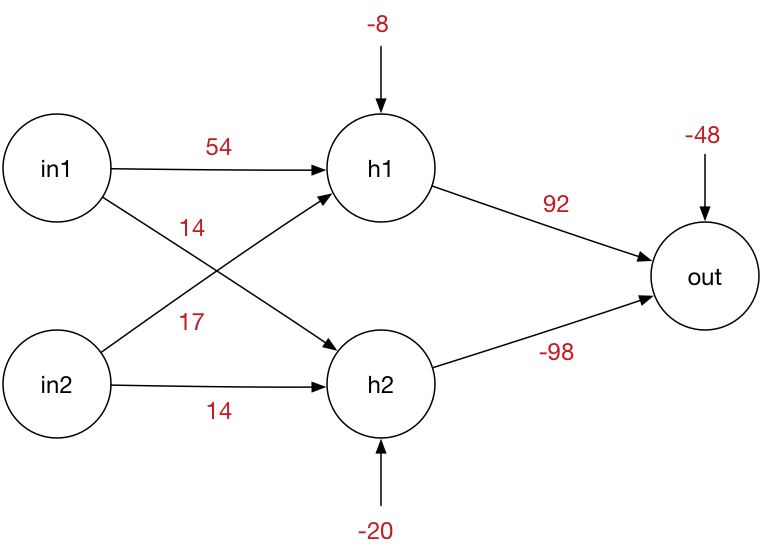
The xor problem can be solved with a neural network with one hidden layer of two nodes and one output node.
The traditional non-linear activation function is the sigmoid function
\[ S(x)= \frac1{(1+\exp(-x))} \]Each hidden node is computed as the linear sum of the inputs (including a constant input of 1), and the weights $\displaystyle\begin{aligned}h_\mathrm{1in}&=w_1^T \begin{bmatrix}\mathrm{in}_1\\\mathrm{in}_2\\1\end{bmatrix} \end{aligned} $ and $\displaystyle \begin{aligned} h_\mathrm{2in}&=w_2^T \begin{bmatrix}\mathrm{in}_1\\\mathrm{in}_2\\1\end{bmatrix} \end{aligned} $
These two equations can be combined into a single matrix calculation for the hidden layers
\[ \begin{bmatrix}h_\mathrm{1in}\\h_\mathrm{2in}\end{bmatrix} = \begin{bmatrix}w_1^T\\w_2^T\end{bmatrix} \begin{bmatrix}\mathrm{in}_1\\\mathrm{in}_2\\1\end{bmatrix} =W_2 \begin{bmatrix}\mathrm{in}_1\\\mathrm{in}_2\\1\end{bmatrix} \]The outputs of the two hidden layers are thus
\[ H_\mathrm{out} = S\left(W_2 \begin{bmatrix}\mathrm{in}_1\\\mathrm{in}_2\\1\end{bmatrix}\right) \]Repeating for the output layer gets
\[ \mathrm{OUT} = S\left(W_1 \begin{bmatrix}H_\mathrm{out}\\1\end{bmatrix}\right) \]This can be done in matlab as
>> S=@(x) 1./(1+exp(-x)); % set up the sigmoid function

>> W2=[54 14 -8;17 14 -20]; % Hidden layer weights

>> W1=[92 -98 -48]; % output layer weights

>> in=[0;0;1]; % trial input (0,0) % in=[1;0;1]; trial input (1,0)

>> H1=S(W2*in); % compute hidden layer outputs

>> Zm=S(W1*[H1;1]); % compute output layer
The figure below shows one of many surfaces that can solve the xor problem with a suitable threshold.

Now most shallow network uses the back propagation algorithm[RHW86][rumelhart1985learning][rumelhart1986learning]. Algorithm adapts the weights so as to reduce the classification errors. (Often called gradient descent)
Algorithm has two parts
Simulated Annealing is an alternative that would allow non-differentiable non linearities, but it is less efficient when compared to the back propagation algorithm.
See papers at end of the pdf version of the lecture notes.
Choi's list was
See paper for more details