SLAM = system location and mapping
Kalman filters are credited to R.E. Kalman but similar algorithms found by T.N. Thiele and P. Swerling. It deals with measurements made on a system such that predictions can be made on the future state of the system. The concept was developed by R.S. Bucy.
The Kalman filter can be seen in action on most GPS satnav systems. As a car enters a tunnel the GPS signal is lost but the satnav will continue to try to maintain the position based on the Kalman filter model.
Variants of the Kalman filter include
It has similarities to the Wiener filter, and is part of a class of algorithms called predictor corrector/ As such variants of the Kalman filter are widely used in SLAM.
Note: The notation here follows that of Welch and Bishop[welch06:_introd_kalman_filter]. http://www.cs.unc.edu/~welch/kalman/
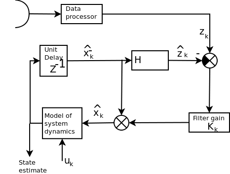
State equations encode the model of the system dynamics. For a linear system $A$ and $B$ are simply constant matrices (this is covered in the third year course state space and frequency methods ) $$x_k = Ax_{k-1} + Bu_{k-1} + Gw_{k-1}$$ Measurement equations, these estimate what you should measure given where you are. $$z_k = {H} x_k + v_k$$
Some assumptions are made on the noise, i.e. that the estimated value of the noise variance has some constant value $E[ww^T]= Q$ (model), $E[vv^T] = R$ (signal), and $E[wv^T] = 0$,
predict the next state from the current state. \begin{equation} \hat{x}^-_k = A \hat{x}_{k-1}+B u_{k-1}\\ \end{equation} predict the covariance of the error in the state estimation. That is, an uncertainty measurement of where you will be. \begin{equation} {P}^-_k = A {P}_{k-1}A^T+ Q_{k-1} \end{equation}
\begin{eqnarray*} K_k &=& {P}^-_k{H}^T_k({H}_k{P}^-_k{H}^T_k + R_k)^{-1}\\ \hat{x}_k &=& \hat{x}^-_k + K_k(z_k- {H} \hat{x}^-_k)\\ {P}_k &=& (I-K_k{H}_k){P}^-_k \end{eqnarray*}
The Kalman filter has two ways to estimate state, the first is 'open loop' relying on perfect knowledge of $A$ and $B$ and any inputs to the system $u$. In this case the Kalman filter gain $K_k$ is zero and the filter applies the normal state space equations. This condition would require $R$ to be large compared with $HPH^T$ approaching infinitely noisy measurements. The second case relies on perfect knowledge of the measurements of the output. If an inverse to $h(x_k)$ or $H$ existed then the state could be recovered as $x=H^{-1}z$. Since this is not normally true the Kalman filter defaults to a modified pseuo-inverse of $H$ and sets the filter gain to $K_k=PH(HPH^T)^{-1}$. Under these circumstances the measurement update equation (in zero noise) becomes $\hat{x}_k = K_kz_k$
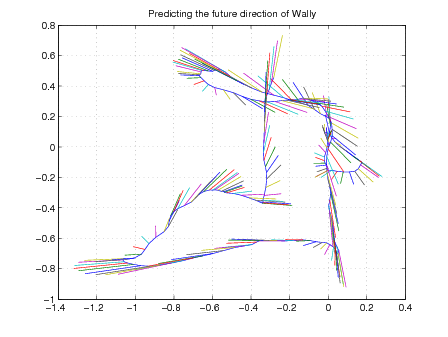
We can use the Kalman filter to predict the movement of a person or robot. The file 'drunkardswalk.m' can be found on blackboard and should run in matlab or octave. The results of a run are shown below.
Forest trails [giusti2016machine]
On the Visual Perception of Forest Trails Istituto Dalle Molle di studi sull'intelligenza artificiale % other=* -Similarities and differences between haptic interfaces and robotics % other=* -Quantification of robot intelligence % other=* -Surgical and medical robotics